Over the next year, I will be completing a research project exploring how biased training data effects the machine learning algorithm of self-driving cars. This project, which I’ll detail in a later post, involves deep neural networks (DNNs), computer vision, linear algebra, and more. Is this project a massive undertaking? Yes. Will that stop me? Absolutely not. Let’s get started.
Neural Network Basics
First, what is artificial intelligence (AI)? AI is a field of computer science pertaining to programming computers so that they demonstrate human-like intelligence.
Machine learning (ML) is a subset of AI that allows algorithms to learn by working on training data before being exposed to real-world problems. Furthermore,** neural networks** (NNs) are a subset of ML that mimics the human brain to make decisions. Most NNs are multi-layered networks that consist of 1 input layer, 1 output layer, and 1+ hidden layers in between. If there are many hidden layers, the NN is considered a** deep neural network **(DNN).
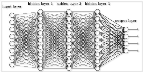
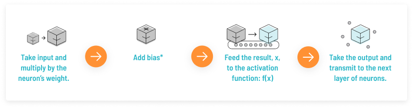
The layers in a NN are made up of neurons that, in short, take in a value and spit out a value. Each neuron in one layer is connected to all the neurons in the next layer. The number of input neurons is the number of features that the NN will work with. In turn, the number of output neurons is the number of predictions that you want the NN to make. The value that a neuron holds is its activation. The activation function of a neuron is an equation that determines whether the neuron should be activated, AKA “fired”, or not. They also help normalize the output of the neurons to be in a small range, usually between 1 and 0 or -1 and 1.
Weights and biases are the parameters that allow a NN to “learn”. Weight affects how much the input will influence the output - how strong the connections between two neurons are. Bias, which stores the value 1, are often added to each layer in a NN to move the activation function left or right. It represents the difference between the function’s output and it’s intended output. Bias serves as a constant that allows the NN to become more flexible and helps control when the activation function will trigger.
**Cost functions **help the network learn which changes matter most and reflects how the network is performing. The cost is small when the network is confident, but large when it isn’t sure what it’s doing. The NN learns by finding the right weights and biases to minimize that cost, this is called gradient descent. Applying gradient descent to the cost function allows the NN to find weights that result in lower error and makes the NN more accurate over time.
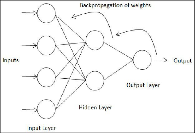
Backpropagation is the process of nudging the weights and biases to decrease cost working from the output layer backwards-after the NN has worked through data. A DNN can loop through its layers using backpropagation: data enters the network through the input layer, is worked on in the hidden layers, and exits through the output layer only to be fed back into the network with updated weights and biases to improve performance.
TensorFlow Basics
TensorFlow is a free software for machine learning, including pre-trained models, datasets, and tutorials. A tensor is a type of data structure, like a vector or matrix, that is basically a multidimensional array.
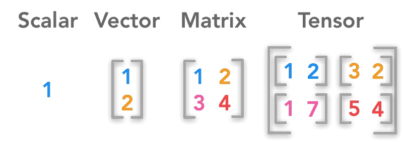
Tensors come in handy when developing ML systems, because they allow you to process large quantities of multi-dimensional data. For example, and image can be defined using three features: hight, width, and color(depth). If you are trying to process images in a NN, like I am, a tensor allows those features to be considered.
Keras is the high-level API used by TensorFlow that provides a Python interface for NNs. To get started with TensorFlow I used Google Colab, which allows you to write and execute python in your browser. Colab is especially useful for people like myself, who work from a small laptop that wouldn’t be able to handle the compute power required when working with DNNs.
Neural Net with TensorFlow-Example
The first NN that I created using TensorFlow is basically the “Hello World” of NNs. It is a pretty common example you’ll see if you research TensorFlow tutorials. Using the MNIST handwritten digit database, I trained a NN to recognize images of numbers using Python:
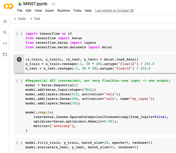
First I imported tensorflow, keras, layers (to create the layers of the NN), and the MNSIT dataset:
<code>import tensorflow as tf
from tensorflow import keras
from tensorflow.keras import layers
from tensorflow.keras.datasets import mnist</code>
Then, I divided the MNIST dataset into training data and testing data, to test/train the NN respectively. Notice that the data is split into x and y values, like a graph. When categorizing an image ML algorithms will view data in a 3- D space and will draw lines between like data points clustered together (hyperplanes) to classify them. Therefore, we need to work with data in that type of space. Since I was working with images I reshaped them to ensure they were all the same size, 28 pixels x 28 pixels, and normalized the data by dividing by 255.
<code>(x_train, y_train), (x_test, y_test) = mnist.load_data()
x_train = x_train.reshape(-1, 28 * 28).astype("float32") / 255.0
x_test = x_test.reshape(-1, 28 * 28).astype("float32") / 255.0</code>
Next I defined the NN to use. Utilizing Keras, I chose a sequential model that is useful when each layer has one input tensor and one output tensor. Sequential models are most likely not the best to classify images, but for the sake of this example it was a simple model to use. To add layers to the NN, I used model.add() and first defined the number of neurons and then the activation function for each layer. I used the relu, or Rectified Linear Unit, activation function which is efficient and allows for backpropogation. Below, line two is the input layer, lines 3-4 are the hidden layers, and line 5 is the output layer.
<code>model = keras.Sequential()
model.add(keras.Input(shape=(784)))
model.add(layers.Dense(512, activation="relu"))
model.add(layers.Dense(256, activation="relu", name="my_layer"))
model.add(layers.Dense(10))</code>
I then specified the training configuration. I defined the loss function, which calculates the error of the NN. I chose the Sparce Categorical Crossentropy (SCCE) loss function, which means that each sample can belong to only one class. I also used the Adam (Adaptive Momentum Estimation) optimizer, which works to find learning rates for each parameter to make the NN more efficient. To track the accuracy of the NN as it learns, I added an accuracy metric.
<code>model.compile(
   loss=keras.losses.SparseCategoricalCrossentropy(from_logits=False),
    optimizer=keras.optimizers.Adam(lr=0.001),
    metrics=["accuracy"],
)</code>
I used the model.fit() and model.evaluate() APIs built into TensorFlow to test and train my NN. model.fit() trained my model by slicing data into batches and iterating over the entire dataset for a set number of repetitions, called epochs. model.evaluate() tested the model using my testing data. The verbose option provided output to my screen as the script ran.
<code>model.fit(x_train, y_train, batch_size=32, epochs=5, verbose=2)
model.evaluate(x_test, y_test, batch_size=32, verbose=2)</code>
Adding more epochs, changing the size and number of layers, and editing the training configuration will help improve the performance of this NN. After this basic NN, working with larger datasets and DNNs is the next step.