In my first Capstone post I gave a rundown of basic AI terms and how to use Tensorflow to create your own machine learning (ML) script.
I’m using Tensorflow to write a script that can process images of roads and determine whether there is an obstacle in the road or not. Since I’m studying self-driving cars, I’d like to see if using biased data to train an object detection script affects the model’s performance. To do this, I’m using a training dataset of clear, bright road images to train a neural network and then testing that script with corrupted images of roads. If the model can’t recognize obstacles in images that are corrupted, then the biased training dataset did have an affect on the model.
Its safe to assume that yes-using biased datasets to train a neural network (NN) will cause the network to function poorly. Its important for NNs to be trained with large, diverse datasets so that they can prepare for unpredictable real-world scenarios. This point has been made in almost any piece of work pertaining to NN. That being said, I’d like to use Tensorflow to create a NN and then test the affects of bias myself. Tensorflow allows for testing and training accuracy of a model to be quantified easily, and you can use python modules to make nifty little graphs that show results.
Its also important to mention that the software of real self-driving cars, like those from Waymo or Audi, are not opensource (no surprise there). So any model created by a novice Tensorflow user like myself is a far cry from the object-detection systems in actual self-driving cars. That being said, the point here is to test how biased training data could affect an object detection system and practice using Tensorflow along the way.
Script Breakdown
The object detection script I wrote using Tensorflow consisted of two datasets (one to train the model and one to test the model), a convolutional neural network (CNN), and a diagram to display the accuracy of the model. The sections of the script are:
- import modules
- create training dataset
- create testing dataset
- standardize the data
- create + compile the model
- data augmentation
- model summary
- train the model
- visualize results
More robust object detection scripts often use bounding boxes (little boxes that surround an item and usually name it) to recognize unique objects in an image. However, my script doesn’t implement bounding boxes and instead classifies images as either having an obstacle, or not.
Import Modules + Datasets
Since I’m using python to write my script, the first step is to import all the modules needed:
import os import PIL import PIL.Image import tensorflow as tf import numpy as np from tensorflow import keras import matplotlib.pyplot as plt from tensorflow.keras import layers from tensorflow.keras.models import Sequential
With that out of the way, I next create my datasets. There are a few ways to approach datasets for your own ML script. Here I will only be discussing datasets of images since thats what I’m familiar with, but other types of datasets do exist. I ended up using Kaggle to write my script, which allows files to be imported from your computer and added to a dataset. The path to that dataset is stored in Kaggle, and can be copied/pasted into your script to be accessed. You can also use Tensorflow’s Google Storage Bucket option to store and reference a dataset, or you can use one of Tensorflow’s own datasets, among other options.
In most ML scripts, you only use one dataset, and use a percentage of it to train the model and the leftover percentage to test (typically 80%train/20%test). If you train and test a model on the same dataset without it splitting into training/testing sections, accuracy metrics will say the model is 100% accurate since you aren’t testing with new data (I learned this the hard way). For my model however, I wanted one testing dataset and one training dataset that could be corrupted later on.
To create the testing and training datasets I used Tensorflow’s “image_dataset_from_directory” option. I first set the image’s height and width so they would all be a uniform size. I also set the batch size, which will I’ll explain later:
batch_size = 32 img_height = 180 img_width = 180
When creating the datasets, you first specify the location of your dataset (in this case, the path that Kaggle provided me). Then, seed provides a random seed for shuffling and transformation. The validation_split represents the percentage of data you want to use to train the model and test the model. Here, a validation_split value of 0.2 means that 80% of the training dataset will be used to train the model and 20% of the testing dataset will be used to test (at this point in time the corrupt images have not been added to the testing dataset, so the two datasets are identical and the split should be used). Finally I then set the subset name, the image sizes, and the batch size.
train_ds = tf.keras.preprocessing.image_dataset_from_directory( "../input/training-dataset", seed=123, validation_split=0.20, subset="training", image_size=(img_height, img_width), batch_size=batch_size)
val_ds = tf.keras.preprocessing.image_dataset_from_directory( "../input/testing-dataset", seed=123, subset="validation", validation_split=0.20, image_size=(img_height, img_width), batch_size=batch_size)
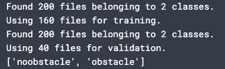
One thing to consider when using data to train a NN is how the model will learn “what is what”. An untrained model can’t make its own conclusions, and piping random images into a model won’t teach it anything. Data should be split into classes of whatever you want to model to learn to differentiate. In my case, I had two classes: “obstacle” and “noobstacle”. In my datasets I included two folders, one for each class, and inside each folder I placed the respective images. I included a line in my script to double-check the classes were being read-in correctly:
class_names = train_ds.class_names print(class_names)
Standardize, Creating and Compiling the Model
Now that the datasets and classes of data are working, the model itself can be created. Like in my first Capstone post, I will be using the Sequential model, relu activation function, and Adam optimizer. However, for this script I have created a convolutional neural network (CNN).
A CNN is a class of deep neural networks, and are commonly used to process images since they resemble the organization of an animal’s visual cortex. CNNs take in tensors of shapes, in this case the image height, width, and an RGB value of 3 (color). These aspects are then assigned importance through weights and biases in order for the model to differentiate one from another.
In Tensorflow, you create a NN through Conv2D and MaxPooling2D layers that each output a tensor of shape. The densest (largest) layers are placed at the top, and the layers shrink as you go down. The number of output channels for each Conv2D layer is controlled by the first argument of that layer. At the end of the model, Flatten and dense layers perform classification by “unrolling” the 3D images into 1D and using what the NN has learned to classify.
To create the CNN the data should first be normalized. This has to do with the mathematics of ML, but this normalization layer basically helps standardize the data.
normalization_layer = layers.experimental.preprocessing.Rescaling(1./255)
Next, I defined the model layers itself:
num_classes = 2
model = Sequential([ layers.experimental.preprocessing.Rescaling(1./255, input_shape=(img_height, img_width, 3)), layers.Conv2D(16, 3, padding='same', activation='relu'), layers.MaxPooling2D(), layers.Conv2D(32, 3, padding='same', activation='relu'), layers.MaxPooling2D(), layers.Conv2D(64, 3, padding='same', activation='relu'), layers.MaxPooling2D(), layers.Dropout(0.2), layers.Flatten(), layers.Dense(128, activation='relu'), layers.Dense(num_classes) ])
In my CNN I added a Dropout layer. This is one of the ways I improved the performance of my model. A Dropout layer randomly sets input to 0 at each layer while training. The inputs that aren’t set to 0 are scaled up by 1. This helps prevent overfitting, which occurs when a model conforms too tightly to training data and doesn’t learn enough to make predictions on new data.
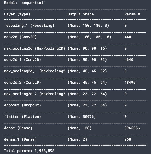
model.summary() helps to visualize what the layers of the CNN look like:
To compile the model I used model.compile:
model.compile(optimizer='adam', loss=tf.keras.losses.SparseCategoricalCrossentropy(from_logits=True), metrics=['accuracy'])
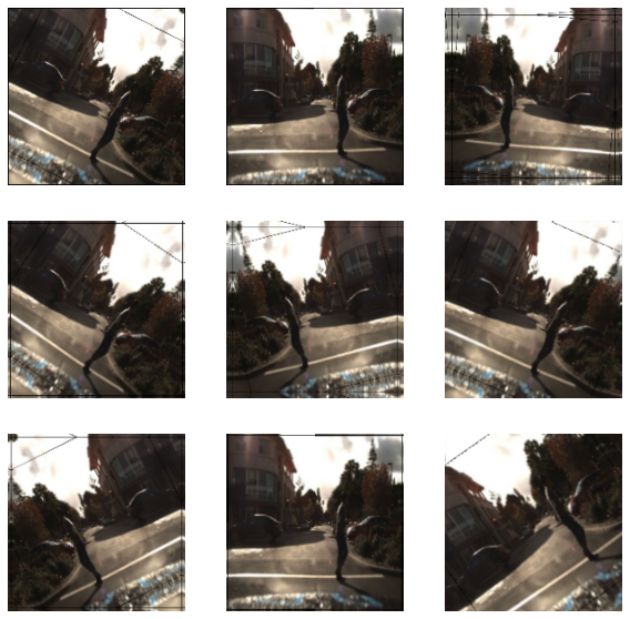
In addition to a Dropout layer, I also used data augmentation to reduce overfitting. Data augmentation makes multiple different images from one training image, by flipping or zooming in on different sections of the image. This helps add in more training data without having to manually add pictures to my datasets.
data_augmentation = keras.Sequential( [ layers.experimental.preprocessing.RandomFlip("horizontal", input_shape=(img_height, img_width, 3)), layers.experimental.preprocessing.RandomRotation(0.1), layers.experimental.preprocessing.RandomZoom(0.1), ] )
Train and Visualize
Training and testing your model with Tensorflow can be done in a few lines of code:
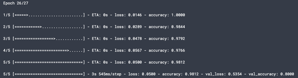
epochs=27 history = model.fit( train_ds, validation_data=val_ds, epochs=epochs )
You’ll notice that here epochs are set to 27. I explained back/forward propagation in my first Capstone post, but epochs are basically the number of times your NN loops through its layers to learn. Batch size, which we set earlier, defines how much of your dataset is put into your model at a time. This is a good way to save computation resources, so you aren’t trying to put a dataset of potentially millions of images into your model at a time.
However, if you set the number of epochs too low, the NN won’t learn enough. If there are too many epochs, the NN can become too familiar with only the training data and overfit when tested. Unfortunately, there is no easy formula to determine how many epochs to use. I just monitored the performance of my NN with different numbers of epochs, and settled on 27.
What can help you determine the number of epochs to use, along with check your model’s accuracy, is visualizing your results. In my script I used matplotlib.pyplot to make a graph.
acc = history.history['accuracy'] val_acc = history.history['val_accuracy']
loss = history.history['loss'] val_loss = history.history['val_loss']
epochs_range = range(epochs)
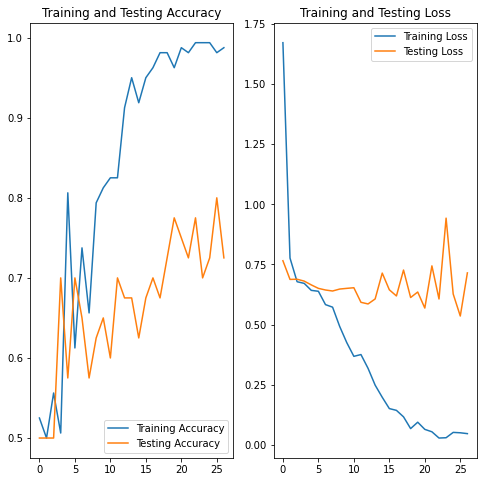
plt.figure(figsize=(8, 8)) plt.subplot(1, 2, 1) plt.plot(epochs_range, acc, label='Training Accuracy') plt.plot(epochs_range, val_acc, label='Testing Accuracy') plt.legend(loc='lower right') plt.title('Training and Testing Accuracy')
plt.subplot(1, 2, 2) plt.plot(epochs_range, loss, label='Training Loss') plt.plot(epochs_range, val_loss, label='Testing Loss') plt.legend(loc='upper right') plt.title('Training and Testing Loss') plt.show()
Wrapping it Up
In this case, the two most important metrics are the training accuracy and the testing accuracy. The training accuracy for my model was nearly 100%, while the testing accuracy was 72-80% (this varied between runs of my script). To put it into perspective, 50% accuracy would be guessing-since the model has only two options to choose from (obstacle or no obstacle). I can live with 72-80% accuracy, although the large difference between my training and testing accuracy means that my model is overfitting. To help fight overfitting, I most likely need to add more images to my dataset (most image datasets have 10,000+ images, mine have 200) or change the type of activation function/optimizer I am using.
From the graph, you can also see that the training loss (prediction error) drastically lowers over epochs, while testing loss doesn’t significantly lower. This is another result of overfitting, although my model does work much better with the inclusion of data augmentation and dropout.
The next step is to edit my model slightly to be more robust, then begin corrupting testing images and experimenting. For now, I have a moderately accurate object detection CNN that would almost certainly cause a real self-driving car to crash, but it works for me.